Why do we need LoRA and QLoRA?
Say I have a pretrained language model and want to adapt it to my own dataset. Maybe I want it to answer questions in a particular domain or follow a specific response format. I can fine-tune it, but how much GPU memory will that take?
With full fine-tuning, we update all the model’s weights. Those weights are only part of the memory bill: training also needs gradients, optimizer states, and intermediate activations. A model that fits on my GPU for inference may still be too large to fine-tune on it.
For a concrete example, a 7-billion-parameter model stored at 16 bits per parameter needs roughly 14 GB just for its weights (using decimal GB). That is before we account for the rest of training. Access to model weights alone does not make adapting them affordable.
This raises two questions. Can we train a much smaller set of parameters? And can we reduce the memory needed to hold the pretrained model itself?
These questions bring us to LoRA (Low-Rank Adaptation) and QLoRA. LoRA keeps the pretrained weights frozen and learns small trainable additions. QLoRA takes this further by combining LoRA with a frozen base model stored in 4-bit precision. We will start with LoRA, then build towards QLoRA. The original papers are linked at the end.
LoRA: Low-Rank Adaptation
What does LoRA set out to achieve?
LoRA’s goal is to adapt a pretrained model while training far fewer parameters than full fine-tuning. Instead of learning a separate change for every entry in a large weight matrix, it represents the change using two smaller matrices.
Think of this as keeping the existing transformation and learning a small correction alongside it. The base weights stay frozen; the correction learns from our dataset. We can apply this to selected linear transformations in a Transformer, such as its attention projections.
How does it work?
Let us zoom in on one linear transformation. Its pretrained weight matrix is W₀, and its input is x. Ignoring bias for simplicity, its original output is W₀x.
LoRA gives the same input a second path, through two trainable matrices called A and B. We add that path’s output to the original output:
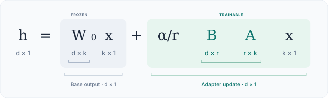
One adapted linear transformation. Only A and B are trained in this diagram; W₀ stays frozen.
The forward-pass formula, with the original LoRA scaling, is:
h = W₀x + (α/r) B(Ax)
Equivalently, the effective weight matrix is:
W = W₀ + ΔW, where ΔW = (α/r) BA
Here is what each symbol means:
| Symbol | Meaning | Shape |
|---|---|---|
| x | Input vector | k |
| W₀ | Frozen pretrained weight matrix | d × k |
| A | Trainable matrix that maps the input to a smaller space | r × k |
| B | Trainable matrix that maps it back to the output space | d × r |
| r | Adapter rank, chosen much smaller than d and k | Scalar |
| α | Hyperparameter controlling the update’s scale through α/r | Scalar |
| h | Output after adding both paths | d |
The order matters: A acts first, then B. Their product BA has the same shape as W₀, so the two transformations can be added. But BA has rank at most r. This is the “low-rank” part: we constrain the update, not the original pretrained matrix.
For example, take a 4096 × 4096 weight matrix. Updating all its entries means training 16,777,216 parameters. With r = 8, A and B together contain only:
(r × k) + (d × r)
= (8 × 4096) + (4096 × 8)
= 65,536 trainable parameters
That is 256 times fewer trainable parameters for this matrix. It does not mean the whole training run uses 256 times less memory: the frozen model and activations still take space. This remaining cost is why quantizing the base model becomes interesting when we get to QLoRA.
How does α/r control adapter strength?
In h = W₀x + (α/r) B(Ax), the base output W₀x has a coefficient of 1, while α/r scales the adapter output. Think of it as a volume knob for the learned correction.
For a fixed A, B, and input x, with r = 8:
| α | α/r | Contribution added to W₀x |
|---|---|---|
| 4 | 0.5 | Half of B(Ax) |
| 8 | 1 | B(Ax) unchanged |
| 16 | 2 | Twice B(Ax) |
A larger scale makes the same adapter update stronger; a smaller scale reduces its contribution. Setting the scale to zero removes the adapter’s contribution entirely.
But α/r = 2 does not mean the adapter is twice as strong as the base model. The relative size of the two contributions also depends on W₀, A, B, and the input. This is an additive correction, not a percentage split between base and adapter.
During training, the scale also affects gradients flowing into A and B. Changing it can therefore change what the adapter learns. Likewise, increasing r changes the adapter’s capacity as well as the denominator, so independently trained adapters at different ranks cannot be compared by α/r alone. The original LoRA paper uses this scaling to reduce the need to retune hyperparameters when varying r.
Where is LoRA applied in a Transformer?
The expression above represents one linear transformation, not an entire Transformer block. A block contains several weight matrices we can choose to adapt:
| Part of the block | Possible LoRA targets | Example module names in Llama-style models |
|---|---|---|
| Self-attention | Query, key, and value projections: Wq, Wk, Wv | q_proj, k_proj, v_proj |
| Attention output | Output projection: Wo | o_proj |
| Feed-forward network (MLP) | Up, down, and, in gated MLPs, gate projections | up_proj, down_proj, gate_proj |
A common starting point is to adapt the query and value projections across Transformer blocks. The original LoRA paper focused on attention weights and found adapting both Wq and Wv effective in its GPT-3 experiments. This is a choice of targets, not a restriction of LoRA.
Each targeted weight matrix gets its own A and B pair. The pretrained weights remain frozen. Targeting more matrices gives the model more trainable capacity, but also increases adapter parameters and training memory. LoRA is not normally attached to the softmax or activation functions themselves; here we are adapting the learned linear projections around them.
Merging LoRA weights for inference
During training, we keep W₀ frozen and learn A and B separately. Once training is complete, we can fold their contribution into a single weight matrix:
W_merged = W₀ + (α/r) BA
This works because BA and W₀ both have shape d × k. At inference time, the two paths become one:
Before merging:  h = W₀x + (α/r) B(Ax)
After merging:   h = W_merged x
These expressions are mathematically equivalent for this linear adapter in evaluation mode, with dropout disabled; floating-point arithmetic can introduce small numerical differences. We do this for each adapted matrix. The merged matrix has the same shape as the original, so inference no longer needs the extra A and B operations. This is how LoRA can avoid additional inference latency after merging.
Merging is optional. Keeping adapters separate lets us store small task-specific checkpoints and swap them while sharing the same base model. A merged checkpoint instead contains the full adapted weights. Keep the original base and adapter files if you want to switch adapters or merge again later.
The base weights are frozen during training; merging afterwards deliberately creates updated inference weights. This simple equivalence assumes ordinary, unquantized linear weights. Merging into a quantized model involves additional precision considerations, which we will revisit with QLoRA.
QLoRA: Fine-tuning a quantized base model
Main contributions
LoRA reduces the number of parameters we train, but the frozen base model still takes up memory. QLoRA combines a frozen 4-bit base with higher-precision LoRA adapters. The paper introduces three memory-saving components: 4-bit NormalFloat (NF4) for storing weights, double quantization for reducing the storage cost of quantization constants, and paged optimizers for handling memory spikes. Let us start with NF4.
NF4: 4-bit NormalFloat
First, how does k-bit quantization work?
Quantization converts values from a representation with more precision to one with fewer bits. For example, we can convert a tensor of 32-bit floating-point values (FP32) into 8-bit integers (Int8). With k bits, we can encode up to 2ᵏ distinct values.
The QLoRA paper’s background section illustrates this with a symmetric Int8 range of [−127, 127]. To use that range, we first scale the input tensor X by its absolute maximum, then round:
absmax(X) = maxᵢ |Xᵢ|

c = 127 / absmax(X_FP32)

X_Int8 = round(127 × X_FP32 / absmax(X_FP32))
       = round(c × X_FP32)
Here c is the quantization scale, stored in FP32. Multiplication and rounding apply elementwise. The largest absolute input maps to magnitude 127, and the other values map proportionally into the integer range. This symmetric example leaves the Int8 value −128 unused.
To dequantize, we divide the stored integers by the same scale:
X̂_FP32 = dequant(c, X_Int8)
       = X_Int8 / c
       ≈ X_FP32
The hat marks reconstructed values. Dequantization restores the original scale, but it cannot recover the precision lost during rounding. For example:
X_FP32 = [-1.0, 0.3, 1.0]
c = 127 / 1.0 = 127

X_Int8 = [-127, 38, 127]
X̂_FP32 = [-1.0, 38/127, 1.0]
        ≈ [-1.0, 0.2992, 1.0]
For this signed symmetric scheme, the general k-bit version replaces 127 with Q = 2ᵏ⁻¹ − 1. The quantized range is [−Q, Q]. An all-zero tensor is handled separately by storing zeros and a nonzero scale, avoiding division by zero.
Blockwise quantization applies the same process to small groups of values, each with its own scale cᵢ. A single large outlier then affects only its block, rather than setting the quantization spacing for the entire tensor. We store both the quantized values and the scales needed to reconstruct them.
Why does the distribution of neural network weights matter?
Uniform spacing gives the tails just as much resolution as the center. But what if most weights are close to zero?
Neural networks commonly start with zero-centered random initialization, using normal or uniform distributions with carefully chosen variance. After training, many weight tensors are still roughly bell-shaped around zero: lots of small values and fewer large ones. The QLoRA paper’s Appendix F examines this behavior in pretrained models. Initialization is part of the background, not a guarantee: trained weights can have outliers, asymmetry, or distributions that differ between layers.
For a zero-centered, bell-shaped distribution, spending the same number of levels on sparse tails as on the crowded center is a poor use of a small codebook. We would like finer spacing where more weights occur.
To compare spacing at 4 bits, let us use a simple uniform codebook with 16 evenly spaced values from −1 to 1:
C_uniform = [-1.0000, -0.8667, -0.7333, ..., 0.7333, 0.8667, 1.0000]
A codebook is a table of reconstruction values; a 4-bit code selects one of its 16 entries. This comparison uses all 16 codes and differs from the signed symmetric integer scheme above, which leaves one code unused. Here the gap between adjacent values is 2/15 ≈ 0.1333.
Take a block whose absolute maximum is 1. Here are a few small positive weights, reconstructed by choosing the nearest value in this uniform codebook or in NF4:
| Original weight | Uniform reconstruction | NF4 reconstruction |
|---|---|---|
| 0.03 | 0.0667 | 0.0000 |
| 0.08 | 0.0667 | 0.0796 |
| 0.16 | 0.2000 | 0.1609 |
| 0.30 | 0.3333 | 0.3379 |
NF4 is closer for the first three examples, while uniform is closer for the last one. The aim is lower error across the distribution, not a win for every value. Our uniform baseline also lacks an exact zero; uniform quantization can represent zero with a different choice of endpoints or zero point. NF4’s distinction is its distribution-aware spacing, not merely including zero.
NF4: Choose the codebook to fit the distribution
NF4 uses 16 nonuniform values, with denser spacing near zero and wider gaps towards the extremes. The values are derived from quantiles of a standard normal distribution. A quantile is the value below which a given fraction of the distribution lies. Equally spaced probabilities give closely spaced values near the peak and more widely spaced values in the tails.
The codebook is fixed and shared; we do not fit a new set of 16 values for each block. Each block gets its own scale instead. NF4 also includes an exact zero, with seven negative and eight positive nonzero values:
C_nf4 ≈ [
    -1.0000, -0.6962, -0.5251, -0.3949,
    -0.2844, -0.1848, -0.0911,  0.0000,
     0.0796,  0.1609,  0.2461,  0.3379,
     0.4407,  0.5626,  0.7230,  1.0000
]
These are reconstruction values, not bin boundaries. When we choose the nearest value, the decision boundary between adjacent entries is their midpoint. The quantile construction motivates the allocation of levels; it does not mean every actual block will place exactly the same number of weights in every bin.
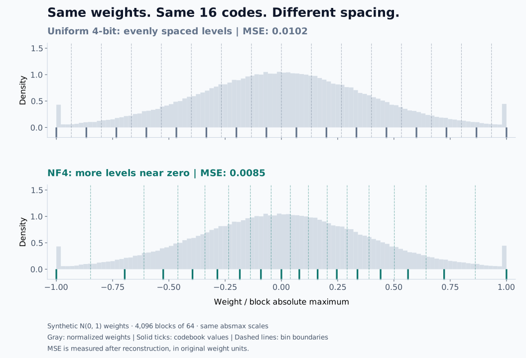
The solid ticks show representable values; dashed lines mark nearest-value bin boundaries. This is just an example using synthetic weights, not a model-accuracy benchmark. Both methods reconstruct the same Gaussian weights using the same block scales. Normalization by each block’s maximum changes the distribution, so the histogram is not itself an exact standard normal density.
Building the NF4 codebook
The paper’s construction uses two adjacent normal-distribution quantiles to choose each representative value. The inverse CDF converts a cumulative probability into a value from the standard normal distribution.
k = 4
num_codes = 2^k
codebook = [] * num_codes

for i = 0 to num_codes - 1:
    p_left  = i / (num_codes + 1)
    p_right = (i + 1) / (num_codes + 1)

    left_value  = inverse_cdf(p_left)
    right_value = inverse_cdf(p_right)

    representative = (left_value + right_value) / 2
    codebook[i] = representative

# Normalize the codebook to [-1, 1].
codebook = codebook / max(abs(codebook))
This shows the construction’s main idea: evenly spaced probabilities become nonuniformly spaced weight values. It is a conceptual sketch: the probability-zero endpoint needs a finite tail cutoff, since inverse_cdf(0) is negative infinity. NF4 also adjusts the positive and negative sets to include an exact zero, giving the 16 values shown above.
Quantizing and dequantizing with the codebook
Once we have the codebook C, quantization is a nearest-value lookup. Apply the following algorithm independently to each block; QLoRA uses blocks of 64 weights.
Quantization takes a block of weights and the shared codebook. It produces 4-bit codes and a scale:
Input: weights[0 .. B-1], codebook C[0 .. 15]
Allocate codes[B]

m = argmax over i of |weights[i]|
scale = |weights[m]|

for i = 0 to B - 1:
    if scale = 0:
        codes[i] = argmin over j of |C[j]|
    else:
        normalized_weight = weights[i] / scale
        codes[i] = argmin over j of |normalized_weight - C[j]|

Output: codes stored as 4-bit values, scale
Here argmax returns the index of the largest absolute weight, while argmin returns the index of the nearest codebook value. The codebook index j ranges from 0 to 15. If two values are equally close, choose the smaller index consistently. For an all-zero block, we select NF4’s exact-zero entry.
Dequantization takes those codes, the block’s scale, and the same codebook. It reconstructs approximate weights:
Input: codes[0 .. B-1], scale, codebook C[0 .. 15]
Allocate reconstructed_weights[B]

for i = 0 to B - 1:
    reconstructed_weights[i] = scale × C[codes[i]]

Output: reconstructed_weights
For example, suppose a block has scale = 2 and contains a weight w = 0.32:
Normalize:    0.32 / 2 = 0.16
Find nearest: C[9] ≈ 0.16093
Store:        code 9, or 1001 in binary
Reconstruct:  2 × 0.16093 ≈ 0.32186
The code is not the weight: 1001 selects entry 9 in the shared codebook, and the block scale restores its magnitude. We store codes plus scales, rather than a high-precision value for every weight.
Finally, 4-bit storage does not mean all arithmetic happens in 4 bits. QLoRA reconstructs the frozen weights in a computation dtype, typically BF16, for matrix multiplication. The adapters remain trainable in higher precision. And the block scales themselves still consume memory—which brings us to double quantization.
Double quantization and double dequantization
NF4 gives us 4-bit weight codes, but each block also needs a scale. Double quantization quantizes those scales too. In the paper’s notation, we store:
- W_NF4: the 4-bit weight codes, in blocks of 64 weights.
- c₂_FP8: the quantized block scales, grouped into blocks of 256 scales.
- c₁_FP32: the second-level scales used to reconstruct c₂.
Before using the weights, we undo these two levels in reverse order. The paper calls this doubleDequant:
doubleDequant(c₁_FP32, c₂_FP8, W_NF4)
    = dequant(dequant(c₁_FP32, c₂_FP8), W_NF4)
    = W_BF16
Read the nested expression from the inside out:
Input:
    W[0 .. N-1]       # NF4 weight codes
    c₂[0 .. M-1]      # Quantized block scales; M = ceil(N / 64)
    c₁[]              # One FP32 scale per group of 256 entries in c₂
    mean              # Mean subtracted from scales before quantization
    C[0 .. 15]        # NF4 codebook

Allocate scales[M]
Allocate weights[N] with dtype BF16

# Recover the scale for each weight block.
for j = 0 to M - 1:
    group = floor(j / 256)
    scales[j] = dequantize(c₂[j], c₁[group]) + mean

# Recover each weight using its block's scale.
for i = 0 to N - 1:
    block = floor(i / 64)
    weights[i] = BF16(C[W[i]] × scales[block])

Output: weights
| Symbol | Meaning | Stored resolution |
|---|---|---|
W[i] | NF4 code for weight i | 4 bits |
C[W[i]] | Normalized NF4 value selected by the code | BF16/FP32 lookup constant |
c₂[j] | Quantized code representing block j’s scale | Typically 8 bits |
c₁[group] | Scale used to decode 256 entries of c₂ | FP32 |
mean | Offset added back after scale quantization | One FP32 scalar per quantized tensor |
scales[j] | Reconstructed scale for weight block j | BF16/FP32 temporary |
The lookup constants are shared across weights, and the reconstructed scales are temporary computation values, not extra per-weight storage.
The paper’s compact formula leaves the stored mean implicit. The result is an approximation of the original weights, not a recovery of the precision lost during quantization.
These reconstructed weights supply the base-model part of the forward pass. Using the paper’s row-vector/batched-input convention, the complete QLoRA expression is:
Y_BF16 = X_BF16 × doubleDequant(c₁_FP32, c₂_FP8, W_NF4)
       + X_BF16 × L₁_BF16 × L₂_BF16
Here L₁ and L₂ are the trainable LoRA matrices; adapter scaling is implicit in this compact expression. This is the same two-branch idea as before, written with X on the left. The base weights stay frozen, and only the adapters receive weight updates. We backpropagate through the reconstructed base transformations to train those adapters; the stored 4-bit weights are not updated.
Where does the 0.373 bits per weight saving come from? Before double quantization, one FP32 scale serves 64 weights. Afterwards, each scale uses 8 bits, plus one FP32 second-level scale shared by 256 of those scales:
Before: 32 / 64 = 0.5 bits per weight

After:  8 / 64 + 32 / (256 × 64)
      = 0.125 + 0.001953125
      = 0.126953125 bits per weight

Saved:  0.5 - 0.126953125
      = 0.373046875 ≈ 0.373 bits per weight
The weight codes themselves remain 4 bits. Including the scale overhead, storage falls from 4.5 to about 4.127 bits per weight, excluding the small mean and other metadata costs. This is a saving in storage per weight, not a reduction in the number of weights.